Introduction
I’ve been experimenting with image generators for a while now and wanted to understand the underlying fundamentals more deeply. I came across this insightful survey paper, Design Fundamentals of Diffusion Models. The paper breaks down the process into three parts: Forward, Reverse, and Sampling Processes. Today, we’re focusing on the Forward Process.
Before delving into the Forward Process, let’s look at a common application: text-to-image generation, and then connect the dots backwards.
Diffusion Models generate images through a process of de-noising (removing noise). A common application of this is text-to-image generation. At a high level, a user inputs text, which is then converted into embeddings. The diffusion model iteratively denoises a completely noisy image using these embeddings as guidance to generate the intended image. State-of-the-art models like Stable Diffusion generate images in a low-dimensional space, called latent space. This is then decoded back into pixel space, resulting in the final image output.
Forward Process (FP)
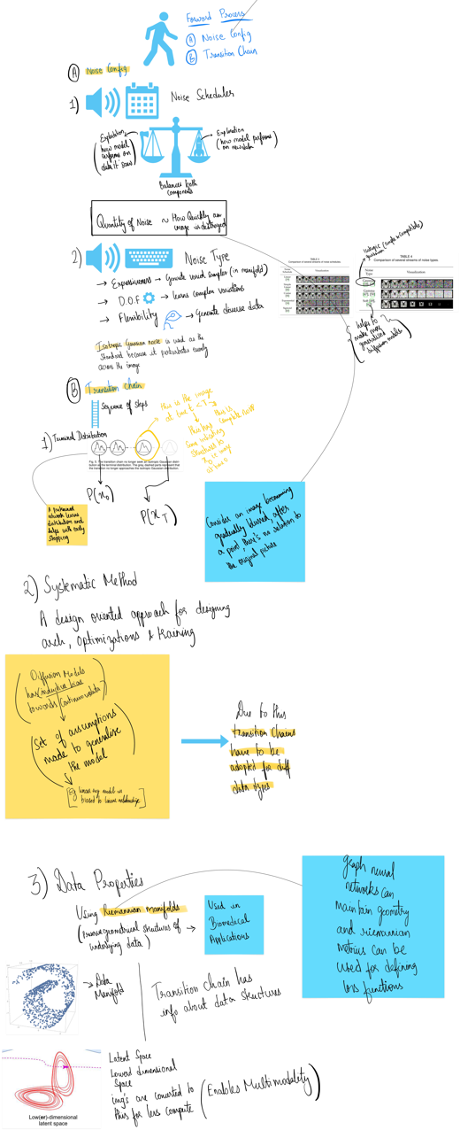
In the Forward Process, noise is continually added to an original image (X₀) in timesteps until we arrive at a completely noisy image (Xₜ). During the Reverse Process, the model tries to denoise the image to reconstruct X₀, which is how the model is trained.
In FP, there are no neural networks involved; noise is progressively added to create noisier versions of the image. The two underlying design components for FP are:
1. Noise Configuration
Noise Configuration can be further broken down into two parts:
-
Noise Scheduler: This controls how noise is added at each timestep, balancing both exploitation (how the model performs on previously seen data) and exploration (how the model performs on new data) capabilities. The quantity of noise added is directly proportional to how quickly an image is degraded, which influences the model’s training time efficiency.
-
Type of Noise: The type of noise chosen affects the model’s capabilities. Isotropic Gaussian Noise is often used due to its uniform distribution, which helps the model generalize better. Key attributes include:
- Expressiveness: Generates varied samples.
- Degrees of Freedom: Learns complex variations.
- Flexibility: Generates diverse data.
2. Transition Chain
This involves the progressive addition of noise to the image, culminating in the terminal distribution (Xₜ). The way this terminal distribution is handled enhances the efficiency of the Reverse Process.
For instance, if we increase the amount of noise quickly to reach the terminal distribution, it speeds up the Forward Process. However, adding too much noise can hinder the Reverse Process, making it difficult for the model to converge or resulting in a noisy output. Therefore, it is crucial to add sufficient noise without completely obliterating the original image’s traceable elements (e.g., consider an image gradually becoming blurred until it’s unrecognizable).
To address this, early stopping is introduced. A pre-trained network learns the distribution and helps select a new terminal distribution that retains basic structures of the original image. This approach ensures the model is generalized while also reducing the time required for the Reverse Process.
-
Systematic Method of Transition Chain Design
A design-oriented approach considers architecture, training, and optimization. This method adapts the transition chain for different data properties:
-
Data Manifolds: Using Riemannian manifolds, which preserve the geometrical structures of the underlying data, can be beneficial, especially in biomedical applications. This can refine the design of the transition chain by better defining the terminal distribution.
-
Latent Representation: Transitioning in latent space, a low-dimensional space, ensures the model learns semantic relationships within the data, enabling multi-modality. Latent features filter out less relevant information, allowing the model to learn abstract, semantic relationships more effectively.
-
Mind Map

